id:mrknさんがベキ分布を生成するRの関数を書いてくれたので、例のやつを書いてみようかと思いました。
> rzipf
function (n, s=1, q=0, supp=c(1,n)) {
  x <- supp[1]:supp[2]
  p <- 1/(x + q)**s
  y <- sample(x, n, replace=T, prob=p)
  return(y)
}
> hist(rzipf(10000),nclass=50,plot=FALSE) hist(rzipf(10000),nclass=50,plot=FALSE)
$breaks
 [1]     0   200   400   600   800  1000  1200  1400  1600  1800  2000  2200
[13]  2400  2600  2800  3000  3200  3400  3600  3800  4000  4200  4400  4600
[25]  4800  5000  5200  5400  5600  5800  6000  6200  6400  6600  6800  7000
[37]  7200  7400  7600  7800  8000  8200  8400  8600  8800  9000  9200  9400
[49]  9600  9800 10000

$counts
 [1] 5958  672  448  280  248  197  157  137  138  120  119   93   78   83   70
[16]   73   63   55   45   60   54   45   48   38   39   37   41   30   45   41
[31]   31   32   24   26   29   33   24   22   16   26   34   26   21   20   26
[46]   20   17   22   19   20

$intensities
 [1] 0.002978999 0.000336000 0.000224000 0.000140000 0.000124000 0.000098500
 [7] 0.000078500 0.000068500 0.000069000 0.000060000 0.000059500 0.000046500
[13] 0.000039000 0.000041500 0.000035000 0.000036500 0.000031500 0.000027500
[19] 0.000022500 0.000030000 0.000027000 0.000022500 0.000024000 0.000019000
[25] 0.000019500 0.000018500 0.000020500 0.000015000 0.000022500 0.000020500
[31] 0.000015500 0.000016000 0.000012000 0.000013000 0.000014500 0.000016500
[37] 0.000012000 0.000011000 0.000008000 0.000013000 0.000017000 0.000013000
[43] 0.000010500 0.000010000 0.000013000 0.000010000 0.000008500 0.000011000
[49] 0.000009500 0.000010000

$density
 [1] 0.002978999 0.000336000 0.000224000 0.000140000 0.000124000 0.000098500
 [7] 0.000078500 0.000068500 0.000069000 0.000060000 0.000059500 0.000046500
[13] 0.000039000 0.000041500 0.000035000 0.000036500 0.000031500 0.000027500
[19] 0.000022500 0.000030000 0.000027000 0.000022500 0.000024000 0.000019000
[25] 0.000019500 0.000018500 0.000020500 0.000015000 0.000022500 0.000020500
[31] 0.000015500 0.000016000 0.000012000 0.000013000 0.000014500 0.000016500
[37] 0.000012000 0.000011000 0.000008000 0.000013000 0.000017000 0.000013000
[43] 0.000010500 0.000010000 0.000013000 0.000010000 0.000008500 0.000011000
[49] 0.000009500 0.000010000

$mids
 [1]  100  300  500  700  900 1100 1300 1500 1700 1900 2100 2300 2500 2700 2900
[16] 3100 3300 3500 3700 3900 4100 4300 4500 4700 4900 5100 5300 5500 5700 5900
[31] 6100 6300 6500 6700 6900 7100 7300 7500 7700 7900 8100 8300 8500 8700 8900
[46] 9100 9300 9500 9700 9900

$xname
[1] "rzipf(10000)"

$equidist
[1] TRUE

attr(,"class")
[1] "histogram"
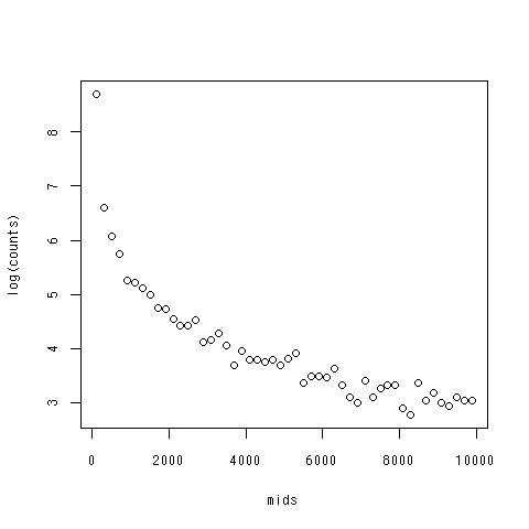
counts <- hist(rzipf(10000),nclass=50,plot=FALSE)$counts
mids <- hist(rzipf(10000),nclass=50,plot=FALSE)$mids
plot(mids,log(counts))
で、できたのがこれ。
何か違う?。適当にやったので間違ってる可能性大!!あとで見直す。